NOW YOU SEE ME, NOW YOU DON’T
The dark art of counting animalsREVIEWER
Sven Rasmussen
Reserves Manager
Sven Rasmussen has worked as an ecologist, land manager and conservationist since 2003. He is passionate about nature and the environment, with a particular interest in and fondness for forests, trees, and wood. A compulsive creator, he enjoys making things both useful and beautiful out of wood and metal.
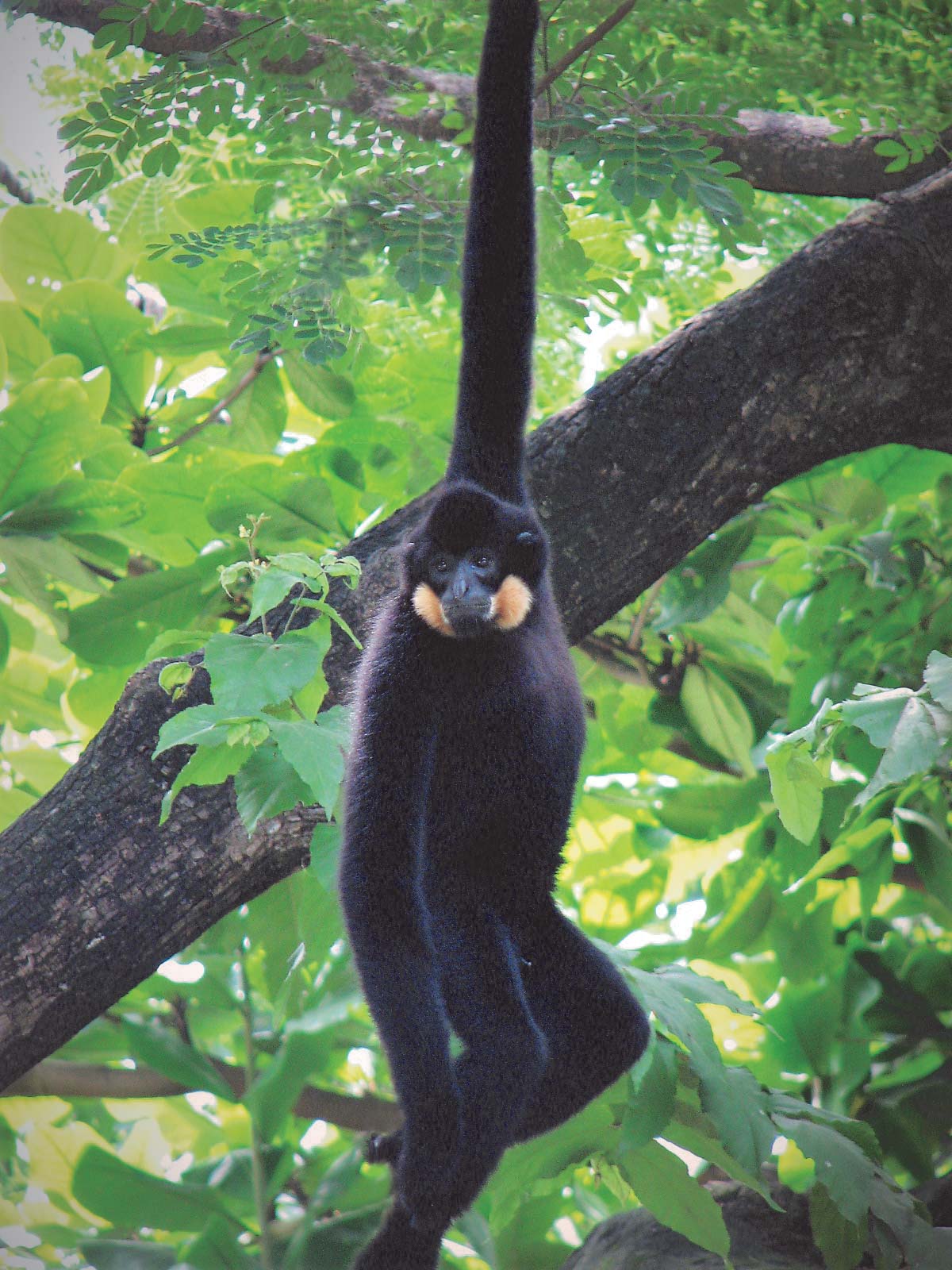
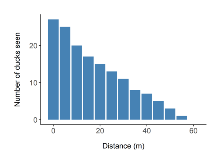
Figure 1. The number of ducks observed at different distances from the transect.
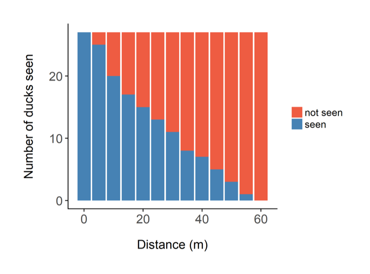
Figure 2. If the blue bars are the ducks you did see, and assuming the animals are randomly distributed with respect to the observer, then the red bars are the ducks that are probably there, but you didn’t see.
AUTHOR

Matt Nuttall
PhD Student
Matt is a PhD researcher at the University of Stirling, where he is investigating how landscape dynamics can be incorporated into spatial conservation planning and landscape-level decision-making, with a particular focus on protected areas. Before starting his PhD, Matt worked as a conservation scientist within the NGO sector in Africa, Asia, and the UK.
Now you see me, now you don’t – The dark art of counting animals
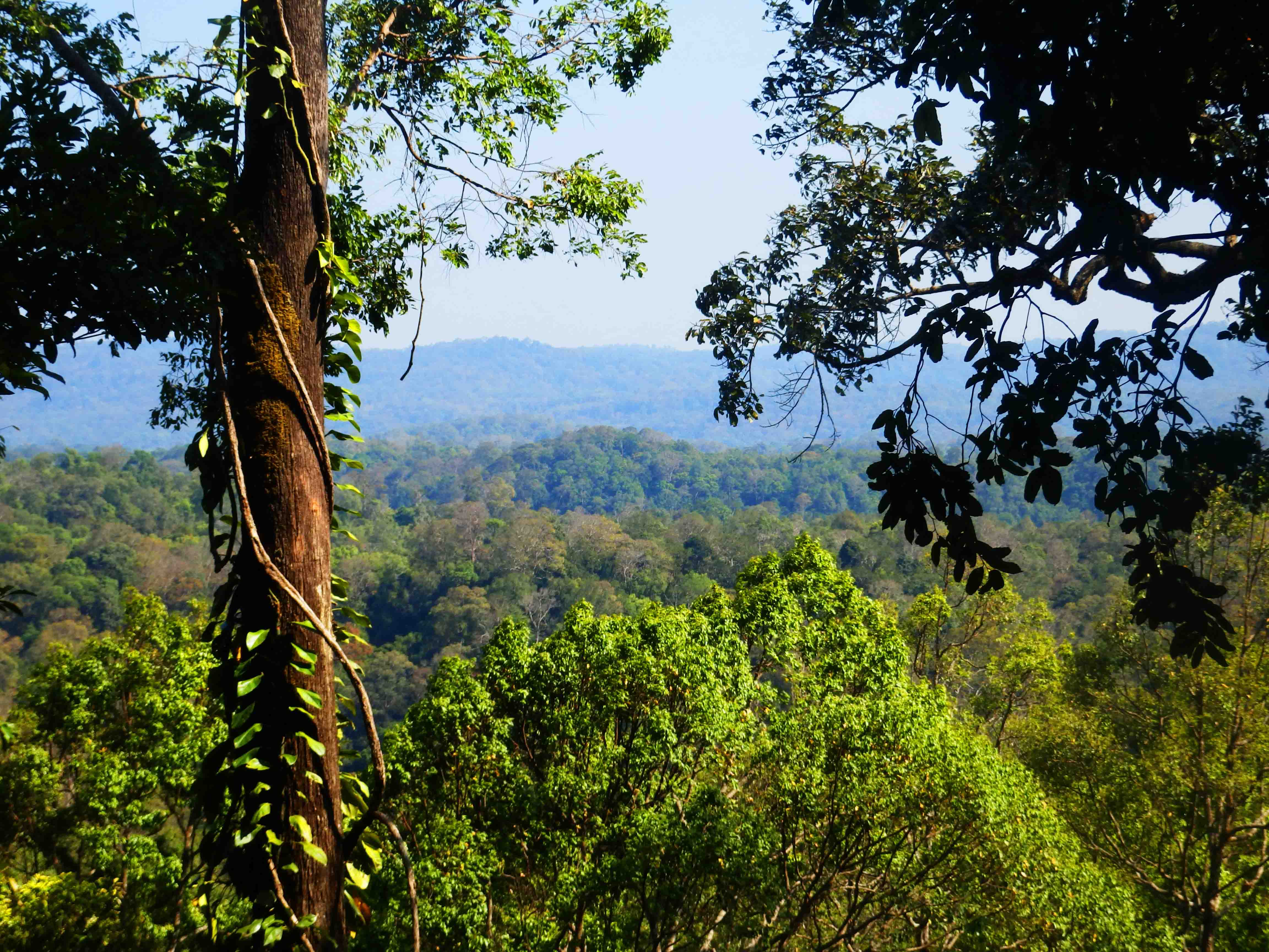
Tropical forests are well known for their spectacular biological diversity, but are under huge pressures from human activities. All across the tropics conservationists work tirelessly on a broad range of interventions to ensure tropical forests are not lost. One of the most important starting points for all conservation interventions is understanding the species or system that we are trying to protect. For species conservation (actions focusing on a single species or group of species), often the most important metric is population size. In fact, it is difficult to know which species are in need of protection without first knowing the trend in population size. This metric continues to be vitally important throughout the life of conservation projects, because it is often the primary indicator of whether our interventions are working. Even in conservation projects which focus on entire landscapes or regions, often some of the best indicators for success (or failure) are the population trends of key species.
If you want to use species population trends as an indicator of project success, you need to actually count the animal or plant! I have spent a lot of my career thus far doing just that – monitoring wildlife populations. I am going to breifly explain methods that are commonly used for counting animals. I am most familiar with methods used for mammals – there are of course amazing methods for monitoring other taxa such as plants and invertebrates, but I don’t have the knowledge to go into them, and so I’m not going to try. Furthermore, I am only going to touch on three of the most widely used methods – this is certainly not an exhaustive review.
Before we get into the methods, it is important to clarify some terminology. When we talk about monitoring the population of a species, we could in fact be talking about several different metrics. Firstly, there is abundance, which just means ‘how many’. Abundance can be broadly split into two categories: 1) absolute abundance which refers to the physical number of animals in the population of interest, and 2) relative abundance: a metric which is linked to absolute abundance, but is of interest as a comparison between different time steps or locations. For example, imagine a population of deer in a small woodland. If you wanted to estimate the absolute abundance of the deer, you would be trying to find out how many individual deer are physically in the woodland, let’s say 35 individuals. To monitor absolute abundance over time, you would need to find out how many individual deer there were at each time step. If you were only interested in relative abundance you don’t want to know exactly how many individual deer there are, you just want to know how many deer there are in year 2, relative to year 1. The next term is density. As the term suggests, this describes the number of individuals of the species in a given area. If you already know the absolute abundance then this is simple. You divide the number of individuals by the area of interest. Let’s take our deer example. We know we have 35 individuals, and the woodland is 5 km2. If we divide 35 by 5 we get 7 individuals per km2. Another important term is distribution. This essentially describes where a species is found. In most cases, when we are interested in distribution we are not asking anything about how many animals there are, we just want to know where they are. This can be a really effective way of monitoring a species over time, as you can see how their distribution changes. More specific than distribution are terms such as occupancy, and area of occurrence. I will go into more detail about occupancy later.
The final term I want to cover is arguably the most important. It is a simple concept, yet is one that is most often overlooked in poorly designed monitoring programmes. The term is probability of detection, and is a fundamental concept in monitoring wildlife. Let’s go back to our woodland example. If you want to count how many deer there are in that woodland, there are many ways you could go about it. But regardless of how you do the actual counting, there is virtually no way of knowing whether you saw and recorded every animal. In reality, it is very difficult to see every individual from a population of wild animals when you are conducting a survey. Therefore you have to assume that the number of animals you saw is an underestimate of the actual number of deer. There is always a margin of error when counting wild animals, because generally speaking, wild animals are elusive and shy, and don’t like being around humans! These traits make the observation and recording of animals particularly challenging. These problems are hugely exacerbated in tropical forests, where the density of the undergrowth means that the visibility for a researcher wandering around looking for animals is really low. So the term probability of detection refers to a number (because it is a probability, it is between 0 and 1), which represents our best guess at the probability that we saw an animal if it was there. To put it simply, this number represents how inaccurate our total count is! If we are able to estimate this probability of detection, then we can apply it to our population estimate and get a corrected (and hopefully more accurate) number.
Moving on to methods. The first method I am going to talk about is called distance sampling. This is arguably the most well-known method for estimating the abundance of mammals. The underlying concept of distance sampling is actually quite simple. I will explain it using a scenario which reflects the origins of the method. Imagine you are conducting a survey of ducks on a lake or river system. The view across the water is obscured in places by emergent vegetation. Now these ducks like to rest and breed in amongst the foliage. We conduct our survey by rowing along transects (or imaginary lines) in boats, and counting the number of ducks we see. All good so far? This is how the surveys have been conducted in the past, and the number of ducks that are seen along the various transects is simply extrapolated to the wider area, thus giving us a total number of ducks. As you go along in your boat though, you notice that you tend to see more ducks closer to the boat, and fewer ducks further away from the boat. You wonder whether the surface vegetation is obscuring your view of ducks further away. You decide to record the distance from the boat to each duck you see, and you plot it on a graph, which might look like Figure 1 on the left.
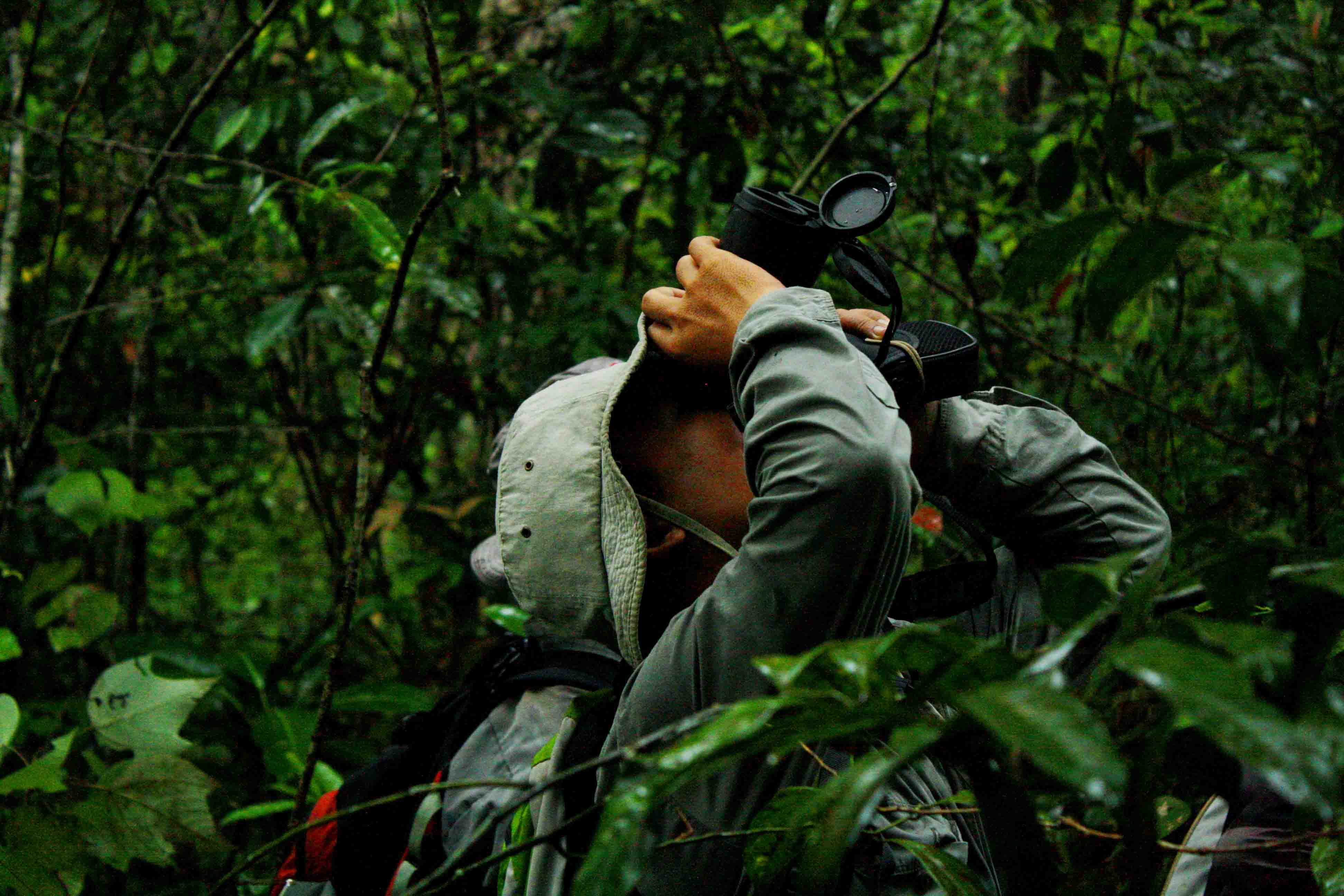
The two most likely explanations for the shape of the graph are either the ducks are genuinely congregating along the transect (in which case your survey design is poor), or your ability to detect them decreases with distance. This second option has been shown to be the case in most wildlife monitoring situations – the further animals are away from you, the more difficult it is to see them. This is the fundamental principle of distance sampling – you use statistical models to estimate the number of animals you did not see. You can then add this to the number you did see, and obtain an estimate of how many animals there are in total (see Figure 2). Distance sampling can be done along transects or at stationary points, depending on the situation. It’s important to be aware that you will have to make several important assumptions, for example that the animals are randomly distributed (in relation to the transects) across the study area, and that the animals do not move in response to the observer (you). You can often deal with assumption violations through careful survey design and having well trained observers. Distance sampling can be an excellent method for monitoring species in tropical forests, because as you can imagine, your ability to see animals at large distances is impaired in thick forests. In some cases though, even distance sampling struggles to provide good estimates because the animals are simply too difficult to see. There have been some exciting advances in using distance sampling for very cryptic species, for example by using auditory cues (the noises the animals make) instead of observations. We trialled this method for gibbons in the forests of Cambodia.
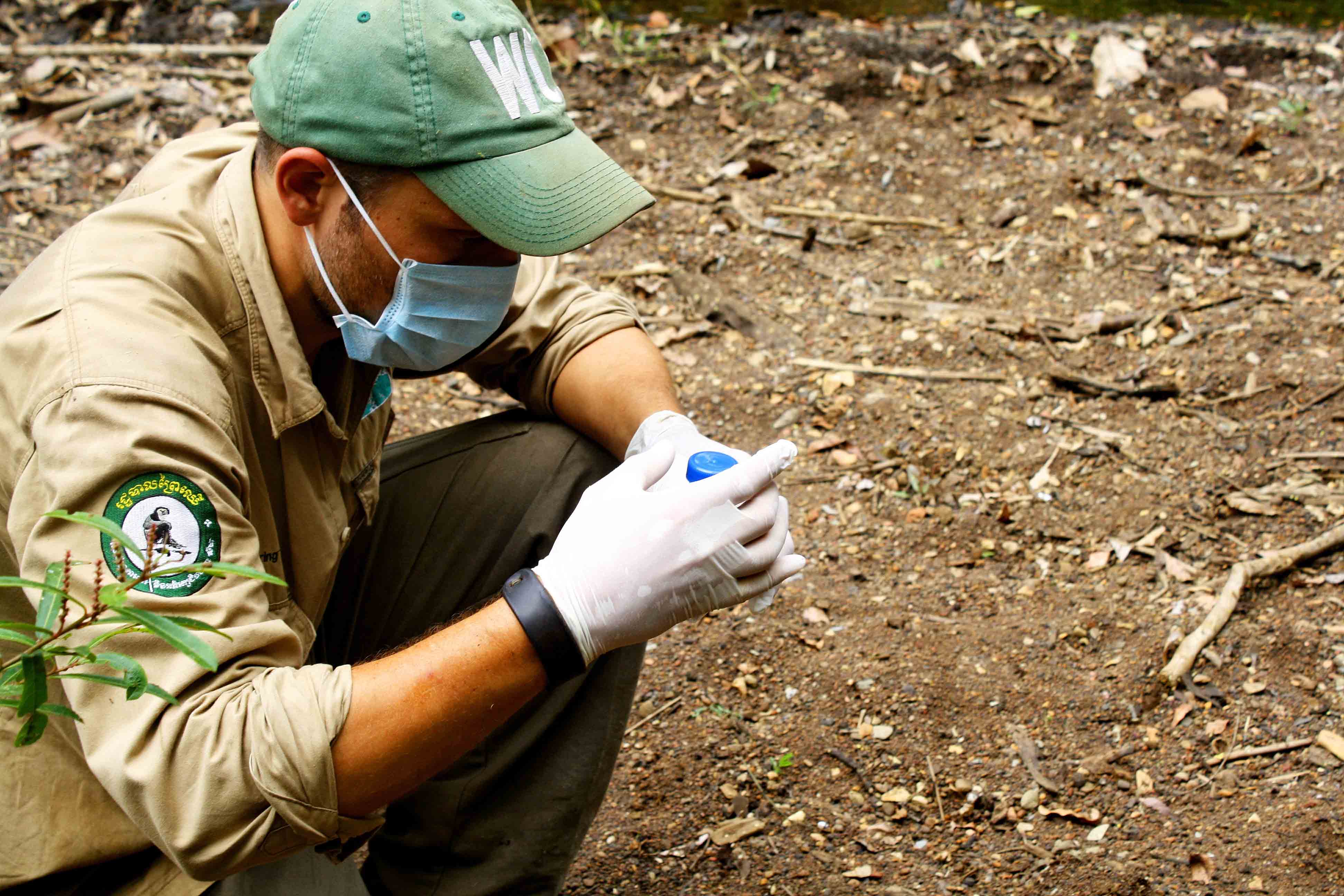
But what if the animal you are trying to count is simply too difficult to observe by walking along a transect or sitting at a stationary point? For example let’s say you are trying to estimate the population size of a nocturnal rodent. Even if you walk along at night with a torch, and are as quiet as possible, you are unlikely to spot any – they are too cryptic! One method you might be tempted to employ is capture-mark-recapture. This method requires you to somehow detect an individual animal, “mark” it (or simply identify it), and then “release” it back into the population. Traditionally this meant actually catching the animal, physically marking it somehow, and then releasing it again. You would repeat this procedure over a number of “sampling occasions”. At each new sampling occasion (each time you catch another set of individuals), if they are unmarked, you mark them and release them. If you catch an individual that is already marked, you take a note of which individual it was and release it again. By repeating this procedure, you end up with a proportion of the total population that are marked. In theory if you continued to do this you would eventually have marked all individuals in the population, and therefore you would know exactly how many individuals there were. This is rare though – most of the time you have to use statistical models to estimate what proportion of the total population you have marked, using amongst other things, the proportion of marked and unmarked individuals that you capture across a given number of sampling occasions. These days capture-mark-recapture studies can be conducted in a variety of ways. Some of the biggest advances have probably been in the ways you can non-invasively “capture” and “mark” animals. In other words, being able to identify individual animals without having to catch them, for example using photographs (often from camera trap images) or DNA (often using hair samples or dung). Other advances include the development of spatially-explicit capture-recapture which uses the information about where you identified a given individual across the different sampling occasions, which provides information about the individuals space use. Capture-mark-recapture also has a set of assumptions which have to be carefully considered, and can mostly be dealt with through careful survey design.
Both of the methods above can be used to estimate abundance and density of an animal population. The final method I will talk about is used to estimate the distribution of a wildlife population. This method is called occupancy. Let’s say we want to estimate the distribution of an endangered frog species, that likes to live around ponds. We have a large survey area that is full of small ponds. It would be impractical for us to survey every pond, and so just like the above two methods, we are going to sample the population. We select a subsection of ponds randomly, and we send observers to each of our selected ponds, or “sites” to try and detect the frog. Now this particular species is very small and difficult to see, but at night they do tend to make very distinctive calls. Our observers are going to walk around the ponds at night and listen out for the calls. If they hear the call, they can record that the species is present. Now remember we are not interested in how many there are, we just want to know if they are there. Therefore once they have heard the frog call, they can record the information and move on to their next pond. After the first visit (or “sampling occasion”) to all of our selected ponds, we have a record of where the frog is present (normally denoted by a “1”), and where the frog is absent (normally denoted by a “0”). Excellent, job done? Not quite!
As you may have guessed, in order to make sure our data is as accurate as possible, we need to account for imperfect detection, as we did in the two methods above. How do we know that we didn’t miss the presence of the frog at ponds where we recorded a 0? Perhaps our observer misidentified a call. Perhaps the frogs at a particular pond simply weren’t calling at the particular time that the observer was there. These are both plausible scenarios, and so to counter these errors (known as false absences) we send our observers back to the ponds several more times where they repeat their survey. This results in each pond having a “detection history” – essentially a set of 1’s and 0’s which we can use to estimate the probability of detecting the frog, given that it is present. What we would probably also do is collect data on some other environmental variables from each pond, normally variables that we think are important for the frogs. In our example perhaps things like pond area, pond depth, and vegetation community might influence whether the frog is present. Using these data and our detection histories, we can use statistical models to estimate the probability that a given pond is occupied by our frog species, thus providing us with really useful information on the distribution of the species. Ideally this survey would then be repeated, perhaps annually, and we would be able to estimate trends in occupancy over time. With these long term surveys, we are also then able to estimate other important population parameters such as the probability of colonisation and probability of extinction, which can be critical for conservationists and managers.
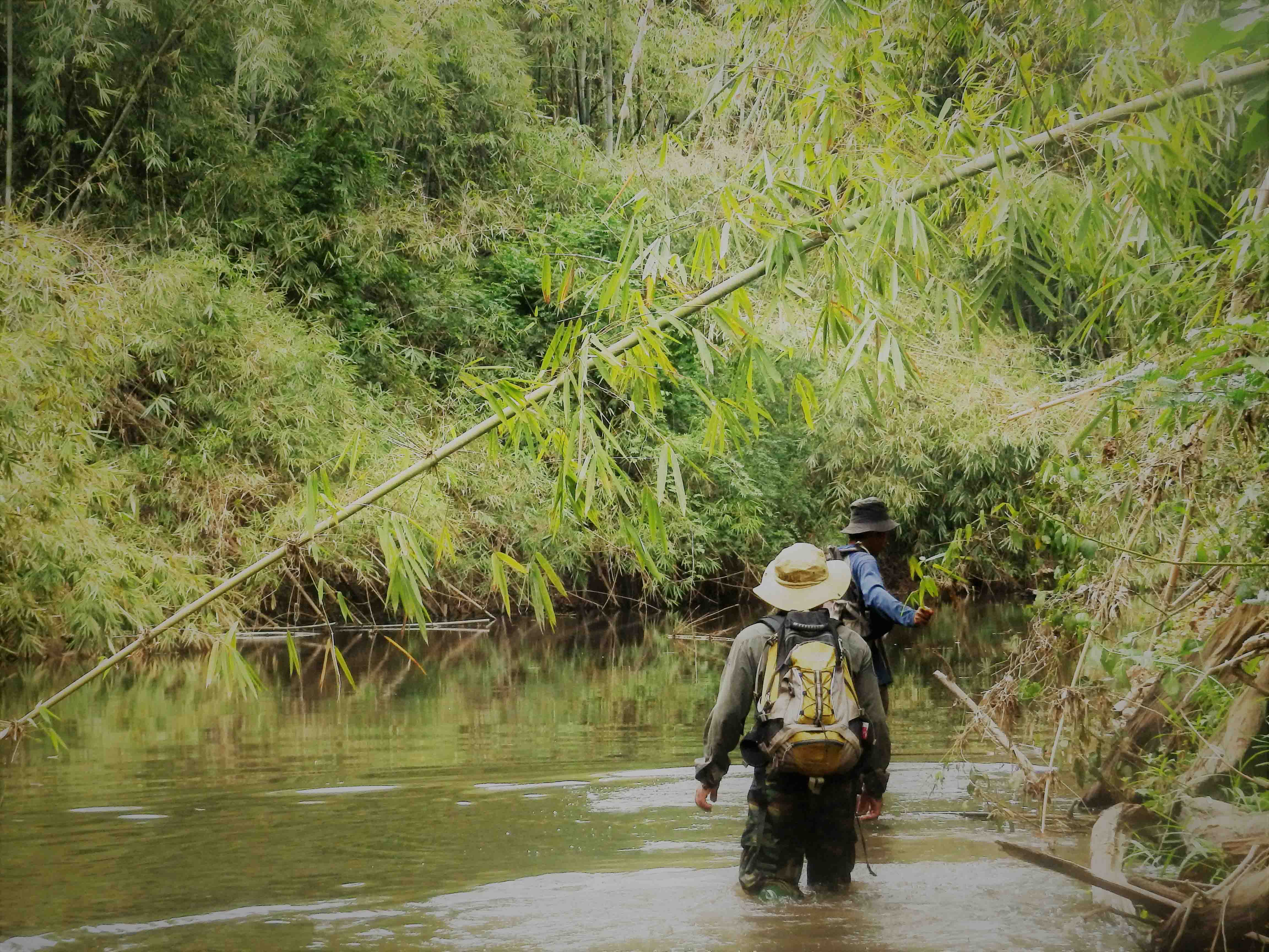
Effectively monitoring wildlife can be challenging, and often is hugely expensive. This is particularly true for monitoring mammals in large tropical forests. Just to put it in perspective, the monitoring program I worked on for several years in Cambodia was based in a national park that was nearly 3000 km2 (700 km2 larger than the Lake District National Park). Our annual monitoring (using distance sampling mostly) took a team of 8 full time employees around 4 – 5 months to complete (just the field work!). Each team member walked between 1200 and 1600 km during the field season, and the program cost tens of thousands of dollars to complete (salaries, vehicles, fuel, equipment etc.). And of course once all the field work is done, there are countless hours of data entry and analysis to be done. But these investments are often extremely good value for money in large conservation projects where perhaps millions of dollars are being spent. The importance of knowing whether your interventions are working cannot be overstated. Every time a visitor or donor came to the park in Cambodia, often the first question about the wildlife was “how many are there?”. Fortunately we could usually answer them, but I doubt they knew the monumental effort that was put into getting those answers. Hopefully next time you ask that question, you will.